With Google Sheets you can track student results and easily visualise how they are progressing.
The most common ways for teachers to visually represent student progress is through graphing the data. However, with conditional formatting in Google Sheets, teachers have another option for graphically representing student progress.
Here’s how to conditionally format your Google Sheet
Step 1: Open up a Google Sheet
Step 2: Enter your students’ details and assessment tasks results
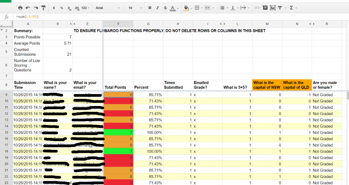
This could be done for you by using Google Forms and self grading assessments. I have used a form that has been auto-marked by the Flubaroo Add-on in Google Sheets – see image above.
Step 3: Set up conditional formatting in your Google Sheet (this isn’t hard)
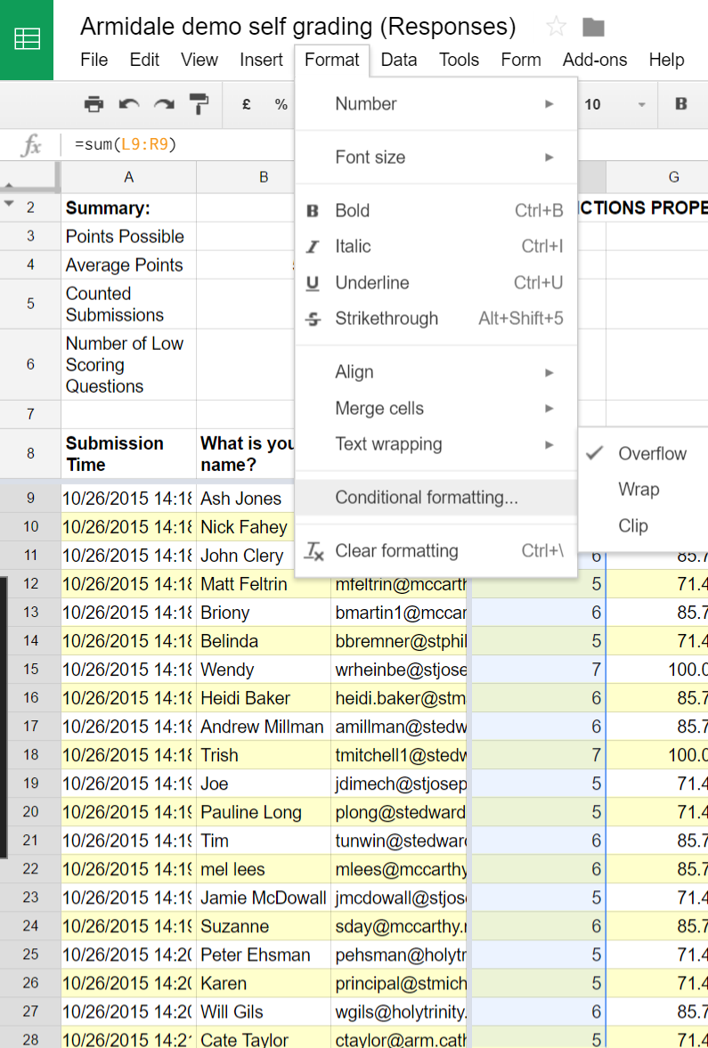
You just need to select the test scores, then click the Format menu and Conditional formatting,
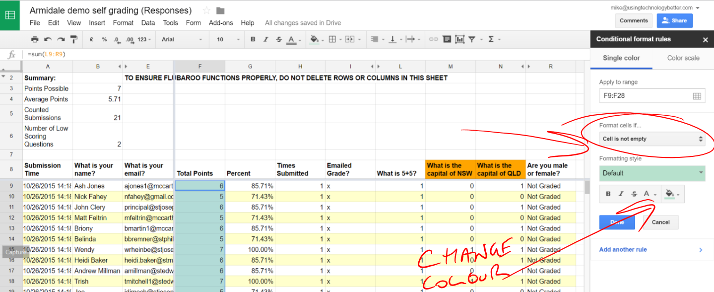
From here, you click on the ‘Format the cells if’ button and set up your condition. If you were working with percentages and you wanted any student who achieved less than 50% highlighted red, you would choose ‘is less than‘ and type in 50. Note that you may want to select is less than or equal to to capture the number as well.
You can add other rules by clicking the Add another rule link.
Here is an example where students who scored 5 or less were highlighted red, between 5 – 6 were highlighted yellow and those that scored 7 were highlighted green.
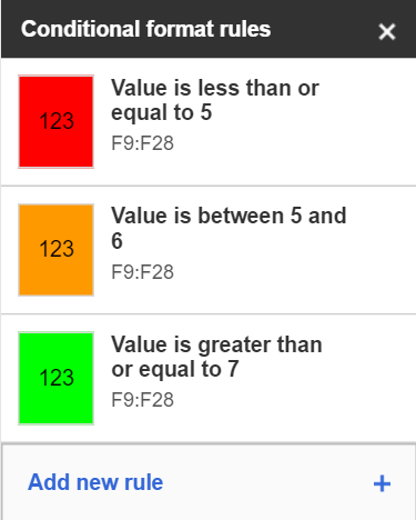
Step 4: After adding all your rules, click Done
Here is an example of a student progress sheet that has been conditionally formatted.

Note: f you copy and paste a cell that has been conditionally formatted, the formatting will be pasted into the new cell and is maintained.
Other Resources
You may also like to explore the grade book template in the Google Sheets template gallery.
In the grade book template for Google Sheets you get:
- An Overview sheet with students progress graphed.
- A marks page linked to a-f grades.
- A student summary graph.
All of these sheets in the Google Sheet are customisable. You can check out the teacher grade book demo here.
.
.
.


