You may have been to a workshop or conference, heard and learnt a vast array of new things and you head back to school full of enthusiasm to implement all that you have learnt. In your head you have all these ideas about how to revolutionise your classroom, until the reality of being back in the classroom hits home. Time tends to fly and good intentions slowly erode.
The key is to implement one thing. It may be small, but take one thing that you have learnt and apply it. It takes time to bring about the changes you imagine. When you hear a keynote speaker they are often condensing many years of trials and experiments into a candy-coated 40 minutes. Don’t be put off by the perceived void between what you are doing and what others tell and show you.
A handy hint is to find something that you normally do and embed it in a digital format. I often suggest finding a task that is repetitive and time consuming and trying to use simple tools to make the workflow better. I like to use the example of a teacher’s grade book. If you haven’t got an integrated LMS at your school, filling in a grade book, collating final marks and trying to see trends quickly is one of the less enviable teaching tasks we face.
In Google Sheets, you can easily make a grade book that is functional and can quickly identify students at risk or those needing extension. Here are 3 things you can try.
1.Use a Template
The easiest way to start the process is to go to Google Sheets and look in the template gallery. Here you will find a grade book template that you can use. It is well designed and allows you to see the progress of each student easily as well as create graphs mapping progress.
2.Build one yourself
Start simply and then build more functions into it as you feel comfortable. In your spreadsheet, start with a column with student names, if you start your list in the second row you can use the first row for headers. Then as you move across you can add marks and calculate percentages by dividing the score received by the total the task is out of. To make a formula in Google sheets that will perform a calculation you want to carry out, just type in ‘=’ and then the formula.
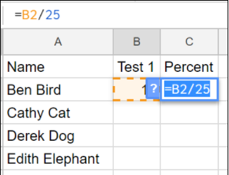 For example, let’s imagine the task is out of 25 and the result of the student is 14. If is entered in cell B2, in cell C3 type =B2/25. This will perform the calculation and display the result of 0.56.
To display this as a percentage, click on the ‘format as percentage’ icon on the top menu bar. You can copy and paste this formula fo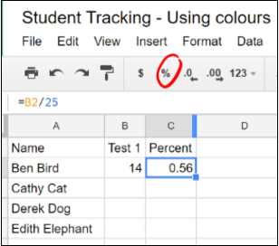 r the rest of the rows.
3.Use conditional formatting to highlight information
When you have several tasks entered and the results are calculated, you can end up with a spreadsheet full of numbers. This can make it hard to visualise the progress of individual students. However, in Google Sheets there is a function called conditional formatting. This allows you to colour a cell based on a condition, like the percentage received. To activate this:
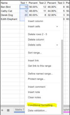
1. Highlight the cells you wish to colour.
2. At the bottom of that menu will be conditional formatting.
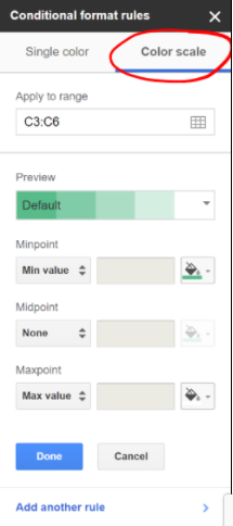
3. Click on that and a menu called ‘Conditional format rules’ will appear on the right hand side of the screen.
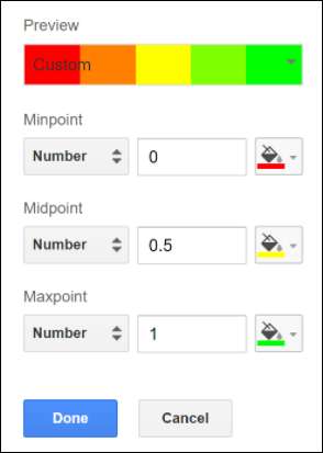
4. The tab on the right allows you to create a colour scale for your results. By default it uses the minimum, median and maximum value to apple shades of green. You can customise this to possibly reflect your data better by changing the Minpoint to be 0, the Midpoint to be 50 and the Maxpoint 100. You are able to assign colours for these settings, red for 0, yellow for 50 and green for 100. This creates a visual snapshot of how each student is progressing.
A simple example of a Grade Book can be accessed via this link.
By taking something that you already do and using the tools in G-Suite, you are able to create a better workflow and, more importantly, visually see trends within your data easily.

